
"Finite Field Arithmetic." Chapter 21A: Extended GCD and Modular Multiplicative Inverse. (Part 1 of 3)
This article is part of a series of hands-on tutorials introducing FFA, or the Finite Field Arithmetic library. FFA differs from the typical "Open Sores" abomination, in that -- rather than trusting the author blindly with their lives -- prospective users are expected to read and fully understand every single line. In exactly the same manner that you would understand and pack your own parachute. The reader will assemble and test a working FFA with his own hands, and at the same time grasp the purpose of each moving part therein.
- Chapter 1: Genesis.
- Chapter 2: Logical and Bitwise Operations.
- Chapter 3: Shifts.
- Chapter 4: Interlude: FFACalc.
- Chapter 5: "Egyptological" Multiplication and Division.
- Chapter 6: "Geological" RSA.
- Chapter 7: "Turbo Egyptians."
- Chapter 8: Interlude: Randomism.
- Chapter 9: "Exodus from Egypt" with Comba's Algorithm.
- Chapter 10: Introducing Karatsuba's Multiplication.
- Chapter 11: Tuning and Unified API.
- Chapter 12A: Karatsuba Redux. (Part 1 of 2)
- Chapter 12B: Karatsuba Redux. (Part 2 of 2)
- Chapter 13: "Width-Measure" and "Quiet Shifts."
- Chapter 14A: Barrett's Modular Reduction. (Part 1 of 2)
- Chapter 14A-Bis: Barrett's Modular Reduction. (Physical Bounds Proof.)
- Chapter 14B: Barrett's Modular Reduction. (Part 2 of 2.)
- Chapter 15: Greatest Common Divisor.
- Chapter 16A: The Miller-Rabin Test.
- Chapter 17: Introduction to Peh.
- Chapter 18A: Subroutines in Peh.
- Chapter 18B: "Cutouts" in Peh.
- Chapter 18C: Peh School: Generation of Cryptographic Primes.
- Chapter 19: Peh Tuning and Demo Tapes.
- Chapter 20: "Litmus", a Peh-Powered Verifier for GPG Signatures.
- Chapter 20B: Support for Selected Ancient Hash Algos in "Litmus."
- Chapter 20C: Support for 'Clearsigned' GPG texts in "Litmus."
- Chapter 20D: "Litmus" Errata: Support for Nested Clearsigned Texts.
- Chapter 21A: Extended GCD and Modular Multiplicative Inverse. (Part 1 of 3)
You will need:
- All of the materials from the Chapters 1 through 15.
- There is no vpatch in Chapter 21A.
- For best results, please read this chapter on a colour display!
ACHTUNG: The subject of the Chapter 21 originally promised at the conclusion of Chapter 20 is postponed. That topic will be revisited later!
On account of the substantial heft of Chapter 21, I have cut it into three parts: 21A, 21B, and 21C. You are presently reading 21A, which consists strictly of an introduction to FFA's variant of the Extended GCD algorithm and its proof of correctness.
Recall that in Chapter 18C, we demonstrated the use of FFA and Peh to generate cryptographic primes, of the kind which are used in e.g. the RSA public key cryptosystem.
We also performed GPG-RSA signature verifications using Peh, and learned how to adapt traditional GPG public keys for use with it.
But why have we not yet seen how to generate a new RSA keypair ?
The still-missing mathematical ingredient is an operation known as the modular multiplicative inverse.
This is a process where, provided an integer N and a non-zero modulus M, we find (or fail to find -- its existence depends on the co-primality of the inputs) the integer X where:
NX ≡ 1 (mod M).
... or, in FFAistic terminology, where FFA_FZ_Modular_Multiply(N, X, M) would equal 1.
In RSA, this operation is used when deriving a public key corresponding to a given private key. (It is also used when ensuring that a selected pair of secret primes has certain properties.) The exact details of this process will be the subject of Chapter 22.
Typically, the modular multiplicative inverse is obtained via the Extended GCD algorithm. It differs from the ordinary GCD of Chapter 15 in that, when given inputs X, Y, it returns, in addition to their greatest common divisor, the Bezout coefficients: a pair of integers P, Q which satisfy the equation:
PX + QY = GCD(X,Y)
The modular multiplicative inverse of N modulo M exists strictly when GCD(N, M) = 1.
Therefore, in that case,
NX + MY = GCD(N,M) = 1
... which can be written as:
NX - 1 = (-Y)M
i.e.:
NX ≡ 1 (mod M).
The reader has probably already guessed that the typical heathen formulation of Extended GCD, i.e. one which uses a series of divisions with remainder, is unsuitable as a starting point for writing FFA's Extended GCD -- for the same reason as why the analogous Euclidean GCD was unsuitable (and rejected) for writing the ordinary GCD routine of Chapter 15. Division is the most expensive arithmetical operation, and it would have to be repeated a large number of times, while discarding many of the outputs (a la the old-style non-Barrettian modular exponentiation of Chapter 6.)
Fortunately, it is possible to write a much more efficient constant-spacetime algorithm for Extended GCD, rather closely similar to the one we used for ordinary GCD.
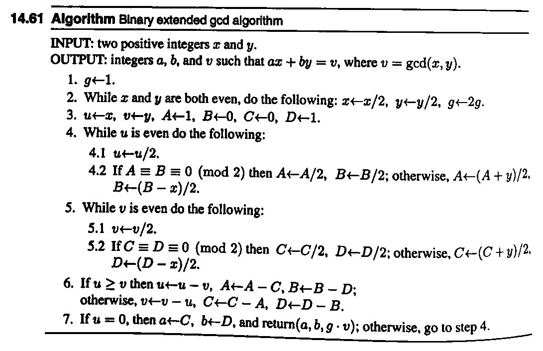
Our algorithm of choice for a properly FFAtronic Extended GCD will be very similar to the Binary Extended GCD pictured in Vanstone's Applied Cryptography.
However, in addition to constant-spacetime operation, our algorithm will differ from the traditional one by avoiding any internal use of signed arithmetic, and will produce outputs having the form :
PX - QY = GCD(X,Y)
Because the Extended GCD algorithm chosen for FFA is not wholly identical to any previously-published one, on account of having to satisfy the familiar requirements, I decided that a full proof of correctness for it ought to be given prior to publishing Chapter 21's Vpatch.
Let's proceed with deriving this algorithm and its correctness proof.
As a starting point, let's take the traditional non-constant-time Stein's GCD given as Algorithm 2 at the start of Chapter 15:
Iterative Quasi-Stein GCD from Chapter 15.
For integers A ≥ 0 and B ≥ 0:
- Twos := 0
- Iterate until B = 0:
- Ae, Be := IsEven(A), IsEven(B)
- A := A >> Ae
- B := B >> Be
- Twos := Twos + (Ae AND Be)
- Bnext := Min(A, B)
- Anext := |A - B|
- A, B := Anext, Bnext
- A := A × 2Twos
- A contains the GCD.
Now, suppose that Twos -- the common power-of-two factor of A and B -- were known at the start of the algorithm, and that it were to be divided out of both numbers prior to entering the loop. The rewritten algorithm could look like this:
Algorithm 1: Quasi-Stein GCD with "Twos" Removal.
For integers X ≥ 0 and Y ≥ 0:
- Twos := Find_Common_Power_Of_Two_Factor(X, Y)
- X := X >> Twos
- Y := Y >> Twos
- A := X
- B := Y
- Iterate until B = 0:
- A := A >> IsEven(A)
- B := B >> IsEven(B)
- Bnext := Min(A, B)
- Anext := |A - B|
- A, B := Anext, Bnext
- A := A << Twos
- A contains GCD(X,Y).
Suppose that we have a correct definition of Find_Common_Power_Of_Two_Factor. (For now, let's merely suppose.)
Algorithm 1 will do precisely the same job as Iterative Quasi-Stein GCD. However, it has one new property -- presently useless -- of which we will later take advantage: because 2Twos (which could be 1, i.e. 20, if either input were odd to begin with) was divided out of X and Y in steps 2 and 3 -- upon entering the loop at step 7, at least one of X, Y can be now relied upon to be odd. (If X and Y were both equal to zero at the start, step 7 is never reached, and the algorithm terminates immediately.)
Now we want to extend Algorithm 1 to carry out Extended GCD.
First, let's introduce two pairs of additional variables. Each pair will represent the coefficients in an equation which states A or B in terms of multiples of X and Y: Ax, Ay for A; and Bx, By for B :
| A | = | AxX - AyY |
| B | = | ByY - BxX |
Elementarily, if we were to give these coefficients the following values:
| Ax | := | 1 | Ay | := | 0 | |
| Bx | := | 0 | By | := | 1 |
... both equations will hold true, regardless of the particular values of A and B.
Of course, this alone does not give us anything useful.
However, if we assign these base-case values to the coefficients at the start of the algorithm, and correctly adjust them every time we make a change to A or B, the equations will likewise hold true after the completion of the loop, and, in the end, it will necessarily be true that:
| AxX - AyY | = | GCD(X,Y) |
... and, importantly, also true that :
| AxX - AyY | = | GCD(X,Y) |
When A or B is divided by two, we will divide each of the coefficients in the corresponding pair (Ax, Ay or Bx, By respectively) likewise by two. When A and B switch roles, the pairs of coefficients will likewise switch roles. When A is subtracted from B, or vice-versa, the respective pairs will be likewise subtracted from one another, keeping the invariant.
In order to keep the invariant at all times, it will be necessary to apply certain transformations. The mechanics of these transformations will account for most of the moving parts of our Extended GCD algorithm.
To make it clear where we will want to put the new variables and the mechanisms for keeping the invariant, let's rewrite Algorithm 1 in traditional branched-logic form:
Algorithm 2. Quasi-Stein with Branched Logic.
- Twos := Find_Common_Power_Of_Two_Factor(X, Y)
- X := X >> Twos
- Y := Y >> Twos
- A := X
- B := Y
- Iterate until B = 0:
- If IsOdd(A) and IsOdd(B) :
- If B < A :
- A := A - B
- Else :
- B := B - A
- If IsEven(A) :
- A := A >> 1
- If IsEven(B) :
- B := B >> 1
- A := A << Twos
- A contains GCD(X,Y).
Now, let's work out what must be done to the coefficients Ax, Ay and Bx, By when we carry out the operations A - B and B - A (steps 9 and 11, respectively) to keep the invariant :
| A - B | = | (AxX - AyY) | - | (ByY - BxX) |
| = | (Ax + Bx)X | - | (Ay + By)Y | |
| B - A | = | (ByY - BxX) | - | (AxX - AyY) |
| = | (Ay + By)Y | - | (Ax + Bx)X |
If we write these simplified expressions side-by-side with the original invariant equations :
| A | = | AxX | - | AyY |
| A - B | = | (Ax + Bx)X | - | (Ay + By)Y |
| B | = | ByY | - | BxX |
| B - A | = | (Ay + By)Y | - | (Ax + Bx)X |
... it becomes quite obvious. In both the A - B and the B - A cases, we only need to compute the sums Ax + Bx and Ay + By ; the only difference will consist of whether they must be assigned, respectively, to Ax, Ay or Bx, By.
Now, suppose we introduce these new parts into Algorithm 2, and end up with :
Algorithm 3. A naive attempt at Extended GCD.
- Twos := Find_Common_Power_Of_Two_Factor(X, Y)
- X := X >> Twos
- Y := Y >> Twos
- A := X
- B := Y
- Ax := 1
- Ay := 0
- Bx := 0
- By := 1
- Iterate until B = 0:
- If IsOdd(A) and IsOdd(B) :
- If B < A :
- A := A - B
- Ax := Ax + Bx
- Ay := Ay + By
- Else :
- B := B - A
- Bx := Bx + Ax
- By := By + Ay
- If IsEven(A) :
- A := A >> 1
- Ax := Ax >> 1
- Ay := Ay >> 1
- If IsEven(B) :
- B := B >> 1
- Bx := Bx >> 1
- By := By >> 1
- A := A << Twos
- A contains GCD(X,Y).
- AxX - AyY = GCD(X,Y).
Unfortunately, Algorithm 3 will not work; the equation at step 30 will not hold true. And the attentive reader probably knows why.
For the inattentive: the erroneous logic is marked in red.
The problem is that we have no guarantee that Ax, Ay or Bx, By are in fact even at steps 22,23 and 26,27 where they are being divided by two. An entire bit of information "walks away into /dev/null" every time one of these coefficients turns out to have been odd. And then, the invariant no longer holds. Instead of correct coefficients Ax, Ay at step 30, we will end up with rubbish.
The pill needed here is known (according to D. Knuth) as Penk's Method. (I have not succeeded in discovering who, when, or where, Penk was. Do you know? Tell me! A reader found the works of Penk.)
This method, as it happens, is not complicated. And it looks like this:
Algorithm 4. Extended GCD with Penk's Method.
- Twos := Find_Common_Power_Of_Two_Factor(X, Y)
- X := X >> Twos
- Y := Y >> Twos
- A := X
- B := Y
- Ax := 1
- Ay := 0
- Bx := 0
- By := 1
- Iterate until B = 0:
- If IsOdd(A) and IsOdd(B) :
- If B < A :
- A := A - B
- Ax := Ax + Bx
- Ay := Ay + By
- Else :
- B := B - A
- Bx := Bx + Ax
- By := By + Ay
- If IsEven(A) :
- A := A >> 1
- If IsOdd(Ax) or IsOdd(Ay) :
- Ax := Ax + Y
- Ay := Ay + X
- Ax := Ax >> 1
- Ay := Ay >> 1
- If IsEven(B) :
- B := B >> 1
- If IsOdd(Bx) or IsOdd(By) :
- Bx := Bx + Y
- By := By + X
- Bx := Bx >> 1
- By := By >> 1
- A := A << Twos
- A contains GCD(X,Y).
- AxX - AyY = GCD(X,Y).
Of course, for our purposes, it does not suffice to merely know what it looks like; we must also understand precisely why it is guaranteed to work !
At this point, the reader should be satisfied with the logic of the Odd-A-Odd-B case; and therefore knows that the invariant in fact holds when we first reach either of the two places where Penk's Method is applied.
Let's start by proving that what Penk does to Ax, Ay (in steps 22..24) and Bx, By (in steps 29..31) does not itself break the invariant.
Review the invariant again:
| A | = | AxX | - | AyY |
| B | = | ByY | - | BxX |
... and see that in the first case,
- If IsOdd(Ax) or IsOdd(Ay) :
- Ax := Ax + Y
- Ay := Ay + X
... the A invariant equation holds :
| (Ax + Y)X | - | (Ay + X)Y | |||
| = | (AxX + XY) | - | (AyY + XY) | ||
| = | AxX | - | AyY | = | A |
And in the second case,
- If IsOdd(Bx) or IsOdd(By) :
- Bx := Bx + Y
- By := By + X
... the B invariant equation holds :
| (By + X)Y | - | (Bx + Y)X | |||
| = | (ByY + XY) | - | (BxX + XY) | ||
| = | ByY | - | BxX | = | B |
The added X and Y terms simply cancel out in both cases.
However, it remains to be proven that Penk's Method actually resolves our problem, rather than merely avoids creating a new one; i.e. that these operations in fact guarantee the evenness of the coefficients prior to their division by two.
Let's demonstrate this for the Even-A case first; later, it will become apparent that the same approach works likewise in the Even-B case.
At the start of step 21, we know that A is even :
- If IsEven(A) :
- A := A >> 1
- If IsOdd(Ax) or IsOdd(Ay) :
- Ax := Ax + Y
- Ay := Ay + X
And, at all times, we know that X and Y cannot be even simultaneously (because we have divided out 2Twos from each of them.)
On top of all of this: since we graduated from kindergarten, we also know about the following properties of arithmetic operations upon odd and even numbers:
Parity of Addition and Subtraction:
| +/- | Odd | Even |
| Odd | Even | Odd |
| Even | Odd | Even |
Parity of Multiplication:
| × | Odd | Even |
| Odd | Odd | Even |
| Even | Even | Even |
So, what then do we know about the parities of the working variables at step 21? Let's illustrate all possible combinations of parities, using the above colour scheme; and observe that we only need the A invariant equation for this. As it happens, there are exactly two possible combinations of parities for its terms :
| A | = | AxX | - | AyY |
| A | = | AxX | - | AyY |
Elementarily, given that A is even at this step, both terms of its invariant equation must have the same parity.
Let's produce a table where all possible combinations of parities of the variables having an unknown parity (Ax, Ay) are organized by the known parities of the variables having a known parity (X, Y, A).
In yellow, we will mark variables which could be either odd or even in a particular combination; in red, those which are known to be odd; in green, those known to be even; and in grey, those for which neither of the possible parities would make the known parities of X, Y, and A in that combination possible, and therefore imply a logical impossibility :
| Odd(X) | Even(X) | Odd(X) | ||||||||||||||||||||
| Odd(Y) | Odd(Y) | Even(Y) | ||||||||||||||||||||
| A | = | Ax | X | - | Ay | Y | Ax | X | - | Ay | Y | Ax | X | - | Ay | Y | ||||||
| Ax | X | - | Ay | Y | Ax | X | - | Ay | Y | Ax | X | - | Ay | Y | ||||||||
Now, let's remove the two impossible entries from the above table:
| Odd(X) | Even(X) | Odd(X) | ||||||||||||||||||||
| Odd(Y) | Odd(Y) | Even(Y) | ||||||||||||||||||||
| A | = | Ax | X | - | Ay | Y | A would be Odd! | A would be Odd! | ||||||||||||||
| Ax | X | - | Ay | Y | Ax | X | - | Ay | Y | Ax | X | - | Ay | Y | ||||||||
And now suppose that we have reached step 23. Therefore we already know that at least one of Ax and Ay is odd. Let's remove from the table the only entry where this is not true; and, finally, in all of the remaining entries, indicate the deduced parity of the variables whose parity was previously indeterminate :
| Odd(X) | Even(X) | Odd(X) | ||||||||||||||||||||
| Odd(Y) | Odd(Y) | Even(Y) | ||||||||||||||||||||
| A | = | Ax | X | - | Ay | Y | A would be Odd! | A would be Odd! | ||||||||||||||
| Ax,Ay are Even | Ax | X | - | Ay | Y | Ax | X | - | Ay | Y | ||||||||||||
All of the parities are now determined.
We are left with only three possible combinations of parities of the terms of A which could exist at step 23. So let's list what happens to each of them when Penk's Method is applied, i.e. Y is added to Ax and X is added to Ay :
| Possible Parity Combos | Parity of Ax + Y ? | Parity of Ay + X ? | ||||||||||||||||
| A | = | Ax | X | - | Ay | Y | Ax | + | Y | = | Even | Ay | + | X | = | Even | ||
| Ax | X | - | Ay | Y | Ax | + | Y | = | Even | Ay | + | X | = | Even | ||||
| Ax | X | - | Ay | Y | Ax | + | Y | = | Even | Ay | + | X | = | Even | ||||
In the Even-A case, Penk's Method works, QED. It is difficult to think of how this could be made more obvious. The parities on both sides of the + sign always match, and so we have forced both Ax and Ay to be even, without breaking the invariant equation for A.
And now, how about the Even-B case ? Suppose that we have reached step 30. Let's do the same thing as we have done for the Even-A case:
| B | = | ByY | - | BxX |
| B | = | ByY | - | BxX |
... does this remind you of anything you've seen before?
Instead of telling the nearly-same and rather tedious story twice, let's leave step 30 as an...
Chapter 21A, Exercise #1: Prove that Penk's Method is correct in the Even-B case.
Chapter 21A, Exercise #2: Why are simultaneously-even X and Y forbidden in this algorithm?
Now, we are ready to rewrite Algorithm 4, this time grouping any repeating terms together, as follows:
Algorithm 5. Extended GCD with Penk's Method and Unified Terms.
For integers X ≥ 1 and Y ≥ 0:
- Twos := Find_Common_Power_Of_Two_Factor(X, Y)
- X := X >> Twos
- Y := Y >> Twos
- A := X
- B := Y
- Ax := 1
- Ay := 0
- Bx := 0
- By := 1
- Iterate until B = 0:
- If IsOdd(A) and IsOdd(B) :
- D := |B - A|
- Sx := Ax + Bx
- Sy := Ay + By
- If B < A :
- A := D
- Ax := Sx
- Ay := Sy
- Else :
- B := D
- Bx := Sx
- By := Sy
- If IsEven(A) :
- A := A >> 1
- If IsOdd(Ax) or IsOdd(Ay) :
- Ax := Ax + Y
- Ay := Ay + X
- Ax := Ax >> 1
- Ay := Ay >> 1
- If IsEven(B) :
- B := B >> 1
- If IsOdd(Bx) or IsOdd(By) :
- Bx := Bx + Y
- By := By + X
- Bx := Bx >> 1
- By := By >> 1
- A := A << Twos
- A contains GCD(X,Y).
- AxX - AyY = GCD(X,Y).
At this point, we have something which closely resembles commonly-used traditional variants of the Binary Extended GCD algorithm. With the not-unimportant difference that all of the working variables stay positive throughout. This way, we will avoid the need to introduce signed arithmetic into the internals of FFA.
Should we proceed with rewriting Algorithm 5 using constant-time operations? ...or is something important still missing? What is it ?
Chapter 21A, Exercise #3: What, other than the use of FFA-style constant-time arithmetic, is missing in Algorithm 5 ?
~To be continued in Chapter 21B.~


Michael A. Penk (with Robert Baillie) factored 2^257 - 1 in 1979. Some of his publications are here.
His resume, on LinkedIn here, includes his contact information and details on his recent work.
Dear bonechewer,
Thank you. I updated the article.
Yours,
-S